Tutorial

In most use cases, clibas is applied to next-generation sequencing (NGS) data derived from genetically encoded libraries (GELs) with a defined design. Examples include mRNA display libraries of macrocyclic peptides or nanobodies, phage display protein libraries, SELEX libraries of foldamer RNA or DNA aptamers, and other GELs.

Such libraries typically contain constant regions and variable regions. The randomized regions may vary in length and composition, but their general architecture (e.g., length) is known. This distinguishes them from datasets such as transcriptome libraries, which do not have a predefined design. Transcriptome libraries can still be analyzed with clibas, but the range of available features is more limited.

After a selection experiment is performed, an enriched library is obtained and its composition is read out by NGS. The task then becomes parsing the sequencing data to understand what happened to the library. How do we remove sequencing artifacts and misamplification products? What sequences are enriched and what is the composition of the library? These are the types of questions that clibas is designed to address.

Building clibas pipelines

At a high level, clibas is all about building analysis pipelines.

A pipeline is an ordered sequence of operations applied to a dataset. Each operation receives data as input and returns data as output, either modified or not. Filtering operations remove reads that fail certain criteria, analysis operations compute statistics and write results to files, and transformation operations modify the data. For example, in silico translation of DNA sequences into peptides is an operation, and plotting the distribution of DNA sequence lengths in a dataset is also an operation.

The principle is simple: every operation takes data in and returns data out.

To build an analysis workflow, operations are enqueued into a pipeline and applied sequentially to the data. The order of operations matters, and the same operation can be used multiple times within a single pipeline. For example, it is possible to analyze the distribution of DNA read lengths immediately after loading the raw data, after performing denoising or filtering steps, or at several points during processing. Because the dataset changes during the pipeline, the results obtained at different stages will naturally differ.

Pipeline operations are accessed through the clibas facade, which also provides the pipeline builder.

To begin, import the package and initialize it with a config file:

import clibas as C
C.initialize(config_path='test_config.yaml')

The .yaml config file typically contains information about the library design, the genetic code, and various hyperparameters such as input and output directories. Details on writing config files are provided in a section below.

A config file is not strictly required. For simple workflows, clibas can also be initialized with default settings and without specifying a library design:

import clibas as C
C.initialize()

Most individual operations are available through C.fastq_parser, which provides tools for parsing .fastq sequencing data, and C.analysis_tools, which enables data analysis. There is also a C.preprocessor module that is primarily used for machine learning workflows; clibas uses it internally when building UMAP–HDBSCAN analyses. Refer to the API reference for a detailed description of each available operation.

Pipeline functionality is accessed through C.pipeline. Operations are added to the pipeline using the enque method:

C.pipeline.enque(
[
    # trim DNA reads
    C.fastq_parser.trim_reads(left='CCAGCC', right='GGTTCTGGC', tol=1),

    # translate DNA -> peptide
    C.fastq_parser.translate(stop_readthrough=False),

    # length analysis of trimmed DNA reads and the resulting peptides
    C.analysis_tools.length_analysis(where='pep'),
    C.analysis_tools.length_analysis(where='dna'),

    # analyze average Phred quality scores
    C.analysis_tools.q_score_analysis(loc=None),

    # discard the peptides of incorrect length (incompatible with library designs)
    C.fastq_parser.len_filter(where='pep'),
]
)

Here, C.fastq_parser.trim_reads(**kwargs), C.fastq_parser.translate(**kwargs), etc represent specific operations described in the API reference. Enqueuing a pipeline constructs the workflow but does not process any data yet. At this stage, clibas checks that the provided hyperparameters and keyword arguments are valid.

To execute the pipeline, a data loader must be specified. The loader will fetch sequencing data and pass it to the pipeline.

loader = C.data_loader.fetch_gz_from_dir(data_dir='./sequencing_data/')
C.pipeline.load_and_run(loader=loader, save_summary=True)

The loader retrieves sequencing .fastq files from the specified directory and feeds them into the pipeline. The data is then passed sequentially through the enqueued operations, each of which processes the dataset and writes outputs as specified. Output files are written either to the directory defined in the config file or to the current working directory.

That’s it – once the pipeline finishes running, the analysis results will be available in the output directory.

Operations on data and library design

A key aspect of building clibas pipelines is understanding how individual operations interact with the underlying data.

Clibas data is organized as a collection of samples, where each sample typically corresponds to a single .fastq file. Each sample contains several associated datasets. When sequencing data is first loaded, two datasets are present: DNA sequences and Q scores. After in silico translation is performed, a peptide dataset is added as well. Each read therefore has a corresponding entry in every dataset: a DNA sequence, a Q score record, and, once translation has been performed, a peptide sequence.

Parser operations can act on any of these datasets. For example, we may want to retain only the reads whose open reading frames (ORFs) produce peptides of a specific length, such as between 14 and 17 amino acids. The operation C.fastq_parser.len_filter accepts a where keyword argument that specifies which dataset the filter should operate on. When filtering based on peptide length, we set where='pep'. The same operation can also be applied to the DNA dataset.

C.fastq_parser.len_filter(where='dna', L_range=[120, 130])

In this example, all reads containing DNA sequences outside the range of 120–130 bp are discarded. Because each read corresponds to entries across all datasets, the associated Q score and peptide records are removed as well. In other words, the entire read is discarded.

Library design

The main feature that enables highly customizable workflows in clibas is the library design abstraction. Clibas is primarily intended for cases where NGS reads originate from designed libraries containing both constant and variable regions. Variable regions may differ in length and composition, but their overall arrangement within the sequence is known.

Information about library design is provided through a library-specific config file (see the section below for writing config files). Designs can be specified for both DNA and peptide sequences using the same general rules.

Randomized amino acids or nucleotides (referred to as tokens) are represented by numerals from 0–9. Tokens that are not subject to randomization (e.g., linker sequences) are represented using the standard one-letter encoding (A, C, T, G for DNA and the standard amino acid alphabet for peptides). A continuous stretch of either randomized or fixed tokens forms a region within the template sequence. Regions are indexed starting from 0.

For example:

    	    seq:      ACDEF11133211AWVFRTQ12345YTPPK
         region:      [-0-][---1--][--2--][-3-][-4-]
    is_variable:      False  True   False True False

Region assignments are generated automatically; only the parent template sequence needs to be specified. In the example above, the library contains five regions, three of which are constant and two – variable.

Numerals used for randomized tokens must correspond to predefined token sets. For instance, an NNK codon encodes all 20 amino acids, whereas an NNC codon encodes only 15. Amino acids derived from NNK codons should therefore be represented by one numeral, and those derived from NNC codons by another. Multiple templates can also be defined to represent libraries with variable regions of different lengths.

A library may contain several sub-libraries. For example, peptides may share the same constant regions but contain variable regions of different lengths. Multiple templates can be used to represent such cases, with the limitation that each template must share the same general topology – the same ordering and total number of constant and variable regions.

For peptide libraries, it is possible (but not required) to provide both DNA and peptide library designs. When both are specified, they must contain the same number of sub-libraries and be listed in the same order. In other words, peptide sub-library 1 should correspond to DNA sub-library 1, and so on. These relationships are defined in the config file, as described in the following section.

Advanced data filtration using library design

With a defined library design, many parser operations can target specific regions within a dataset. This allows filtering criteria to be applied selectively to particular regions of a sequence.

For example, it is possible to enforce strict Q score thresholds within variable regions while tolerating lower Q scores in constant regions. In such a case, a Q score filter can be applied to selected regions only:

C.fastq_parser.q_filter(loc=[1, 3], thresh=30)

This operation discards all reads that contain Q scores below 30 in regions 1 and 3 of the DNA library.

More sophisticated filtering strategies are also possible. For instance, a cr_filter operation can remove reads whose peptide sequences contain excessive mutations within constant regions. The filter can be applied to specific regions and configured to tolerate a limited number of mutations.

C.fastq_parser.cr_filter(where='pep', loc=[0, 2], tol=2)

This operation discards reads whose peptides contain more than two mutations across constant regions 0 and 2 combined. Peptides containing two or fewer mutations across those regions are retained.

Suppose that mutations are not tolerated at all in region 4. A second filter can be added:

C.fastq_parser.cr_filter(cr_filter(where='pep', loc=[4], tol=0))

Together, these operations retain only those peptides that contain at most two mutations across regions 0 and 2, and no mutations in region 4. In this way, highly specific filtration strategies can be constructed by combining multiple operations.

Other common operations available from C.fastq_parser include in silico translation of DNA sequences into peptides, trimming DNA reads, filtering sequences based on variable region composition, and removing ambiguous reads (such as DNA sequences containing N base calls). The API reference provides a complete list of available operations.

Because pipeline operations can reference individual regions, the order in which operations are applied is important. For example, a peptide may contain ambiguous amino acids (encoded as _ or + by clibas) in one of its constant regions. This can occur if the sequencer assigns an "N" base call, resulting in an ambiguous codon that cannot be translated to a single amino acid. Suppose a peptide contains _ in constant region 0. If we first apply an operation such as C.fastq_parser.filt_ambiguous(where='pep'), which removes reads containing ambiguous (_) in peptide sequences, and then truncate peptide sequences to a specific region (for example, using C.fastq_parser.fetch_at(where='pep', loc=[2])), the peptide will be removed. However, if these operations are applied in the opposite order, the peptide will survive, since the ambiguity is lost after the fetch_at step. This illustrates that pipeline order can directly affect results; filtering operations are not commutative.

Writing config files

Config files in clibas are written in .yaml format, and are used to specify library designs, in silico translation behaviour, and various runtime settings such as output directories and logging behavior. Several reference config files used in jupyter notebook examples are available on github.

Library design

Library design is the most important component of a config file. It defines the structure of the sequencing library and allows parser operations to target specific regions within reads.

A library design consists of two parts: templates and monomer sets.

Templates are parent strings that describe the structure of each sub-library. Randomized tokens are represented by numerals (0–9), while constant tokens are written using the standard alphabet (A, C, T, G for DNA, or the standard amino acid alphabet for peptides). Monomer sets define which bases or amino acids correspond to each numeral.

An example DNA library design is shown below:

LibraryDesigns:
  dna_templates:
    - "CACTATAGGGTTAACTTTAAGAAGGAGATATACATATG112112112112112TGCGGCAGCGGCAGCGGCAGCTAGGACGGGGGG"
    - "CACTATAGGGTTAACTTTAAGAAGGAGATATACATATG112112112112112112TGCGGCAGCGGCAGCGGCAGCTAGGACGGGGGG"
    - "CACTATAGGGTTAACTTTAAGAAGGAGATATACATATG112112112112112112112TGCGGCAGCGGCAGCGGCAGCTAGGACGGGGGG"
    - "CACTATAGGGTTAACTTTAAGAAGGAGATATACATATG112112112112112112112112TGCGGCAGCGGCAGCGGCAGCTAGGACGGGGGG"
    - "CACTATAGGGTTAACTTTAAGAAGGAGATATACATATG112112112112112112112112112TGCGGCAGCGGCAGCGGCAGCTAGGACGGGGGG"
    - "CACTATAGGGTTAACTTTAAGAAGGAGATATACATATG112112112112112112112112112112TGCGGCAGCGGCAGCGGCAGCTAGGACGGGGGG"

  dna_monomers:
    1: ["A", "G", "T", "C"]   # N
    2: ["G", "T"]             # K

The dna_templates entries correspond to sub-libraries, as described in the previous section. Each template describes the layout of constant and variable regions within the sequence. The dna_monomers dictionary defines the possible tokens associated with each numeral. In this example, 1 corresponds to the degenerate base N, and 2 to K.

A library design may include multiple templates in order to represent libraries with variable region lengths. However, all templates must share the same topology – that is, the same ordering and number of constant and variable regions.

Designs can be specified at either the DNA level, the peptide level, or both. When both are provided, the templates must correspond to each other: dna_templates[0] should describe the DNA sequence that produces pep_templates[0] and so on. Peptide designs are specified using the analogous fields pep_templates and pep_monomers.

Providing a library design is optional, but many parser operations rely on this information. For example, an operation such as

C.fastq_parser.cr_filter(where='pep', loc=[0, 2])

requires knowledge of region boundaries. If no library design is specified, operations that reference specific regions will raise an error.

For some applications (e.g., SELEX), only DNA-level design makes sense – it is not necessary to supply both DNA and peptide.

Advanced library design patterns

The distinction between constant and variable regions is a modeling convention and not a strict rule. In some libraries, certain positions within a nominally constant region may be functionally critical, while others may tolerate variation. The library design system is flexible enough to represent such cases.

For example, a typical mRNA display library of cyclic peptides might be encoded with a design like this: y1111111CGSGSGS, where y is a custom initiator amino acid used for peptide cyclization with a downstream cysteine C. The cysteine residue (C) is therefore essential. We may wish to ensure that all analyzed peptides contain this cysteine, while allowing variability in the neighboring region (GSGSGS). This can be achieved by defining the cysteine position as a randomized token set that permits only one amino acid:

LibraryDesigns:
  pep_templates:
    - "M11111112GSGSGS"

  pep_monomers:
    1: ["A", "C", "D", "E", "F", "G", "H", "I", "K", "L", "M", "N", "P", "Q", "R", "S", "T", "V", "W", "Y"]
    2: ["C"]

In this configuration, token 1 corresponds to any proteinogenic amino acid, while token 2 encodes cysteine exclusively. C.fastq_parser.cr_filter(where='pep', loc=[1], sets=[1, 2]) can then be used to ensure that every read contains C where encoded.

The same strategy can be used to divide, merge, or redefine regions as needed. By adjusting templates and monomer sets, complex library architectures can be represented in a systematic way. The only structural constraint is that no more than ten distinct randomized token sets (0-9) can be defined within a single design.

Translation configuration

Config files can also specify how DNA sequences should be translated into peptides. This is primarily useful when working with non-standard genetic codes, which are common in mRNA display selections where genetic code reprogramming is frequently used.

If no translation table is provided, clibas assumes the standard E. coli genetic code.

A custom translation table can be defined as follows:

constants:
  translation_table:
    ATA: "I"
    ATC: "I"
    ATT: "I"
    ATG: "r"
    ACA: "T"
    ...

In this example, "r" represents a non-canonical amino acid. The translation_table should define all 64 codons.

Many mRNA display selections also modify the initiator amino acid used at the start of an open reading frame. This can be specified as:

constants:
  custom_ini_aa: "Y"

During in silico translation, clibas by default searches for ATG codons to initiate ORFs. The start of translation can be constrained further by specifying a custom ORF locator, defined as a regex that must match the DNA sequence before translation begins:

FastqParserConfig:
  orf_locator: "AGGAGA.......ATG"

In this example, translation will only begin if a Shine-Dalgarno sequence (AGGAGA) is present upstream of the start codon. If the pattern is not found in a read, the translation operation will return an empty ORF.

Optional chemical representations

When performing UMAP-HDBSCAN analyses, clibas can optionally use RDKit fingerprints of amino acids or nucleotides to better capture chemical similarity between tokens. In this case, the chemical structures of token (amino acids below as an example) can be provided using SMILES strings.

constants:
  aa_SMILES:
    A: "N[C@@H](C)C(=O)"
    C: "N[C@@H](CS)C(=O)"
    D: "N[C@@H](CC(=O)O)C(=O)"
    r: "N[C@@H](CCCNC(CF)=N)C=O"   #non-canonical amino acid
    ...

If this section is omitted, UMAP-HDBSCAN analyses can still use simple one-hot encoding.

Output and logging configuration

Config files can also control output directories and logging behavior.

TrackerConfig:
  logs: "./outputs"                  # Directory for writing logs to
  parser_out: "./outputs"            # Directory that stores fastq parser outputs
  analysis_out: "./outputs/analysis" # Directory that stores outputs of data analysis operations
  
LoggerConfig:
  verbose: true                      # Verbose loggers print to the console
  log_to_file: false                 # Write logs to file
  level: "INFO"                      # Logger level; accepted values: "DEBUG", "INFO", "WARNING", "ERROR"

TrackerConfig specifies where different outputs are written. Parser outputs and analysis results can be directed to separate directories if needed.

LoggerConfig controls the behavior of the logging system. Logs can be printed to the console, written to files, and filtered by severity level (DEBUG, INFO, WARNING, or ERROR).

Data analysis tools

The package provides a range of tools for analyzing data during processing. These methods are accessed through C.analysis_tools and behave like other pipeline operations such as those in C.fastq_parser. This means they can be added directly to pipelines and executed at any stage of the workflow. Analysis operations may be queued before, after, or in between filtering steps, and the same operation can be queued multiple times if needed.

Examples of available analyses include summarizing sequence length distributions, computing token frequencies, generating WebLogo-style plots, evaluating library convergence, gathering Q-score statistics, and counting reads. The complete list of available operations is described in the API reference.

Many C.analysis_tools operations accept the same where and loc keywords used by C.fastq_parser. These arguments allow statistics to be computed for specific datasets (e.g. where='pep' or where='dna') or particular regions of the sequence (loc=[1, 3], etc.).

UMAP–HDBSCAN data visualization and clustering

A useful analysis feature built into the package is UMAP–HDBSCAN visualization and clustering. Dimensionality reduction using UMAP is commonly used to visualize high-dimensional sequence data, while HDBSCAN provides an unsupervised clustering method that can be applied on top of UMAP embeddings.

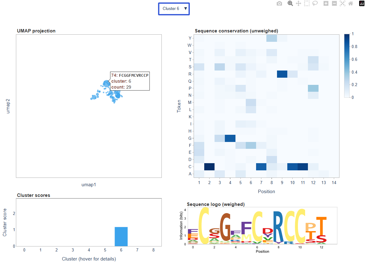
Within clibas, sequences from individual samples can be embedded into a two-dimensional UMAP space and subsequently clustered using HDBSCAN. The resulting visualization is written as an HTML dashboard, which can be used to explore the structure of the dataset. Sequences with similar composition tend to cluster together in the embedding. Points representing sequences are plotted as circles whose size reflects read count, while color indicates the cluster assigned by HDBSCAN:

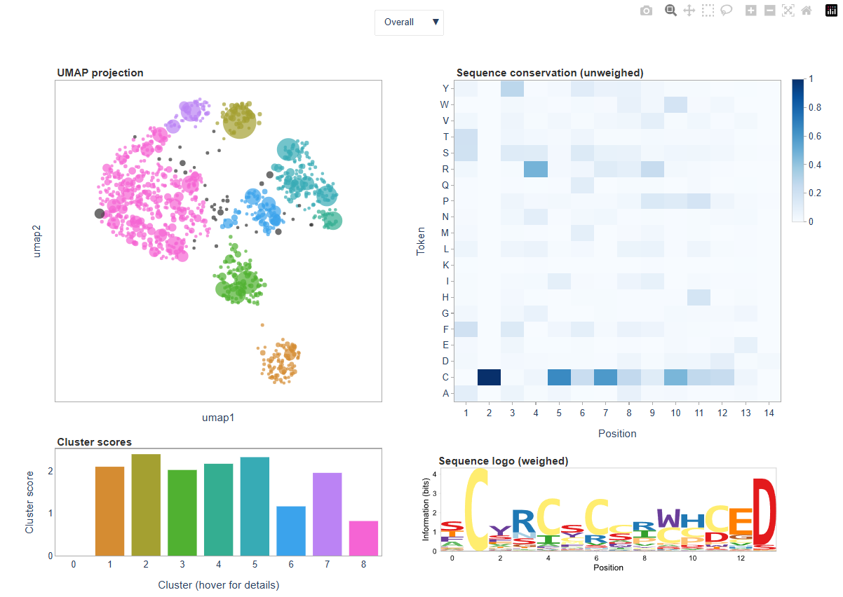
The dashboard is interactive; for example, we can explore sequence convergence in a particular cluster, and get sequence information for a particular datapoint by hovering over it:

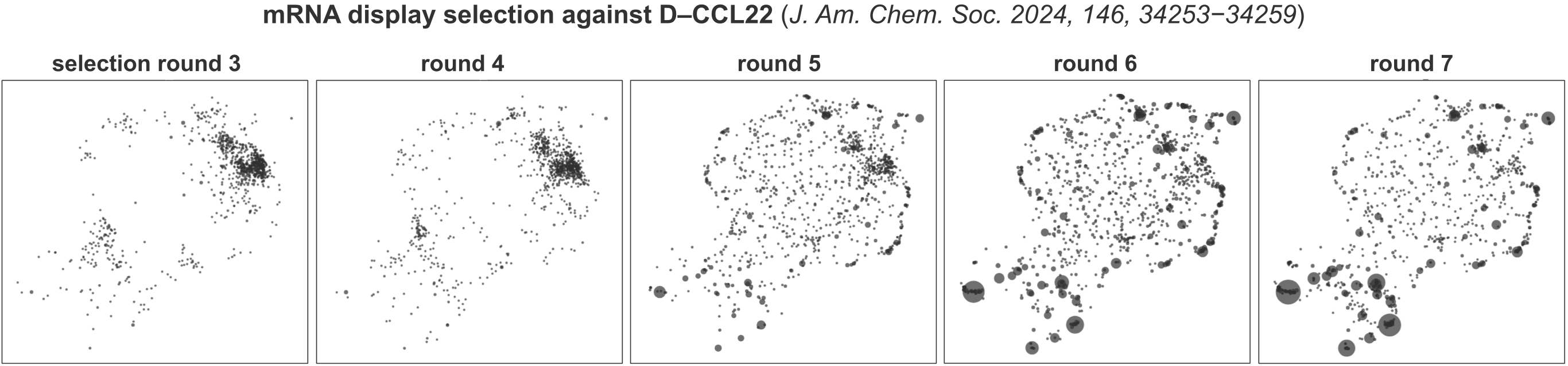
UMAP embeddings are inherently stochastic, meaning that repeated runs on the same dataset will produce different layouts. To facilitate comparison between related samples (for example, positive and negative samples from the same experiment), the operation can be called with single_manifold=True. In this mode, sequences from all samples are embedded onto the same manifold, allowing the same peptide or DNA sequence to appear in the same region of the embedding across datasets. This greatly facilitates visual comparison. Below aresingle_manifold=True UMAP embeddings for the data from J. Am. Chem. Soc. 2024, 146, 34253−34259, which show an mRNA display library composition evolved during affinity selection against D-CCL22:

Both peptide and DNA datasets can be analyzed using UMAP–HDBSCAN. The dataset to analyze is selected using the where keyword. Because embedding and clustering can be computationally expensive for large datasets, the top_n parameter can be used to restrict the analysis to the most abundant sequences. For large datasets, values between 1000 and 5000 sequences typically work well.

Before embedding, sequences must be converted to a numerical representation. This is controlled by the F parameter. If F=None, sequences are encoded using a simple one-hot representation, which generally works well for most applications. Alternatively, users may specify F='pep_ECFP4', which represents amino acids using RDKit fingerprints derived from their chemical structures in a manner described in ACS Cent. Sci. 2022, 8, 814–824 and Nat. Chem. 2021, 13, 992–1000. This encoding can capture chemical similarities between amino acids more effectively.

If F='pep_ECFP4' is used and the peptides contain non-canonical amino acids, the config file must define chemical structures for all amino acids in the alphabet using the aa_SMILES field (see the config section above).

An example UMAP-HDBSCAN operation is shown below:

C.data_analysis.umap_hdbscan_analysis(
    top_n=2000,
    where='pep',
    F='pep_ECFP4',
    single_manifold=True
)

Performance and Memory Usage

The library is written in numpy and is generally optimized for speed. The table below shows execution times for a typical pipeline run on a dataset containing 8.85M initial reads.

Operation	Time [s]	Dataset size [million reads]	Processing speed [million reads/s]
fetch_dir_gz	19.6	8.85	0.45
translate_dna	43.3	8.85	0.20
length_summary	3.3	8.85	2.67
q_score_summary	6.8	8.85	1.31
fastq_count_summary	5.5	8.85	1.62
length_filter	3.9	4.40	1.12
constant_region_filter	0.9	4.35	4.64
variable_region_filter	11.8	4.23	0.36
q_score_filter	1.7	2.50	1.47
fetch_region	0.2	2.50	10.70
filter_ambiguous	7.7	2.50	0.33
sequence_level_convergence_summary	6.6	2.50	0.38
token_level_convergence_analysis	10.0	2.50	0.25
unpad_data	7.7	2.50	0.32
save_data	0.0	2.50	58.21
fastq_count_summary	2.7	2.50	0.94
library_design_summary	0.1	2.50	36.27
umap_hdbscan_summary	52.4	2.50	–
Total	184.2

A dataset of 8.85M reads is processed in ~3 minutes, including UMAP-HDBSCAN clustering. In silico translation is the slowest operation (aside from UMAP–HDBSCAN analyses, whose runtime varies depending on the dataset). Nonetheless, translation runs at roughly 0.2 million reads per second, although the exact speed depends on ORF length.

By default, all operations are performed in memory. Sequences (DNA, Q scores, and peptides) are stored as byte strings, so each token takes one byte of memory. This is typically sufficient for datasets containing fewer than ~10 million reads, depending on the available RAM. For larger datasets, memory usage can become limiting. To accommodate different dataset sizes, clibas provides three data-loading strategies.

The first option loads all files into memory at once:

loader = C.data_loader.fetch_gz_from_dir(data_dir='./sequencing_data')

C.data_loader.fetch_gz_from_dir fetches all .fastq.gz files from data_dir and loads them into memory simultaneously. This is convenient when analyzing multiple samples that share the same library design.

The second option processes files sequentially:

streamer = C.data_loader.stream_from_gz_dir(data_dir='./sequencing_data')

C.data_loader.stream_from_gz_dir loads .fastq.gz files from data_dir one at a time. When used with the pipeline runner

C.pipeline.stream(streamer, save_summary=True)

the pipeline analyzes each file sequentially, reducing peak memory usage.

Finally, for very large datasets, clibas can stream reads in chunks from a single file:

streamer = C.data_loader.stream_from_gz_file(
    fname='./sequencing_data/example.fastq.gz',
    reads_per_chunk=1e7
)

This loader reads a specified number of sequences (reads_per_chunk) into memory at a time. Each chunk is then processed by the pipeline as a standalone sample before the next chunk is loaded.

At present, clibas assumes single-end reads; paired-read matching is not implemented. If paired reads must be merged, external tools such as FLASH are recommended prior to analysis. Read trimming, however, is supported directly and can be efficiently performed using:

C.fastq_parser.trim_reads()